老师,我太想写SLAM了-李群/李代数篇
本篇论文主要以“A micro Lie theory for state estimation in robotics”这篇论文为基础,简单介绍下李群李代数在SLAM中的应用。与以外介绍不同的是,本篇更多的是在介绍在于求导Jacobian方面,希望能更快地帮助同学们克服SLAM状态估计过程中的求导难题,进而能快更好地写出自己的算法,加速研究进度。
前言
SLAM的一个核心问题是估计由位置(3DOF)和姿态(3DOF)组成的6DOF刚体运动。对于研究者来说,不同论文/系统中对方向的定义差异和旋转矩阵本身不可求导的特性都会给学习过程带来较大的困扰。对于前者来说,通常在论文第三章的开始部分,都会给出定义是World->Body还是Body->World,然后对于后者来说,研究者通常会用欧拉角、四元数或李群等方式来对位姿进行参数化表示。
欧拉角表示除了本身具有的万向锁问题外,也会因为旋转顺序的不同导致求导过程中特别复杂,这个在loam_velodyne的实现中尤为明显。四元数的表示存在JPL和Hamilton两种表示情况,其中经典算法OpenVINS采用的是基于JPL的旋转表示,VINS-Mono采用的是Hamilton的数学表示。表明上看,两种表示方法不同仅仅是方向的不同(JPL通常表示的是World->Body,而Hamilton表示的是Body->World,似乎更适用于机器人学),但数学上两种表示方式也各有各的缺陷及其对应的优化解决方案,具体可看知乎上wuRDmemory的解析、泡泡邱笑晨的四元数误差传播和Joan Sola的Quaternion kinematics for the error-state Kalman filter这三篇文章,相信你读完后就有自己的理解和答案。
鉴于前面两种表示方法现在已经有很多blog解析,所以我们就着重探讨基于李群/李代数的位姿表示。本篇Blog中,我们将以Joan Sola的a micro lie theory for state estimation in robotics
第一章 机器人学中的李群/李代数的基础定义.
为了保证行文逻辑通顺,我们在这里将简要回顾下李群/李代数的基础概念。如前文所述,我们将不再对于李群和李代数之间的关系进行深入探讨,而更多的讨论基于群下的机器人运算。从数学上来看,机器人是喜欢李群的原因是,群可以通过的映射关系找到对应的向量空间,从而保证位姿本身的特性。如基于旋转的群即是\(SO(3)\),对应的是\(\mathfrak{so(3)}\)李代数。基于旋转加位姿的群是\(SE(3)\),对应的李代数是\(\mathfrak{se(3)}\)。基于旋转加位姿加速度的群\(SE_{2}(3)\),对应的李代数是\(\mathfrak{se_{2}(3)}\)。在我粗浅的理解\(SE_{2}(3)\)群最大的好处是可以解决滤波中的可观性问题,我们会在滤波的章节再进行深入理解,在本篇blog中将不做过多的讨论,更多精力将放在\(SO(3)\)和\(SE(3)的讨论上\)。那么首先,我们来回顾下什么是群。
1.1 群.
如
\end{aligned} \end{equation}
\begin{equation} \begin{aligned} &\text{结:}(\mathcal{X} \circ \mathcal{Y})\circ \mathcal{Z} = \mathcal{X} \circ (\mathcal{Y} \circ \mathcal{Z})
\end{aligned} \end{equation}
\begin{equation} \begin{aligned} &\text{幺:} \mathcal{E} \circ \mathcal{X} = \mathcal{X} \circ \mathcal{E} = \mathcal{X} \end{aligned} \end{equation}
\begin{equation} \begin{aligned} &\text{逆:}\mathcal{X} \circ \mathcal{X}^{-1} = \mathcal{X}^{-1} \circ \mathcal{X} = \mathcal{E} \end{aligned} \end{equation}
$$
我们把满足上述的群画出来,则其拓扑表示应该如下所示:
观察拓扑表示,我们就会发现,群上每一个点都是一样的。这些约束让群成了一个光滑的表面。我粗浅的微积分知识告诉我,在这种情况下,原本在欧式空间中不可导的旋转矩阵通过转换变成了局部可微了。由于光滑是函数可微的重要条件,所以李群也常常被人们叫光滑流形(以上为个人记忆方法,并不一定符合数学严谨性,如果有问题欢迎讨论和拍砖)。
在机器人中,无论2D还是3D应用。李群具有将集合元素变化,并进行旋转、平移、缩放以及他们任意组合的操作能力。则 $$ \begin{equation} \begin{aligned} SO(n)&: \hspace{1em} \text{旋转矩阵} \hspace{1em} \mathbf{R} \cdot \mathbf{x} \triangleq \mathbf{R}\mathbf{x} \end{aligned} \end{equation}
\begin{equation} \begin{aligned} SE(n)&: \hspace{1em} \text{欧式矩阵} \hspace{1em} \mathbf{H} \cdot \mathbf{x} \triangleq \mathbf{R}\mathbf{x} + \mathbf{t} \end{aligned} \end{equation} $$
这里的$n$表示的是维度。当$n=2$时,表示的是2D空间下的机器人运动,当$n=3$时,表示的是3D空间下的机器人运动。
1.2 切向量空间和李代数.
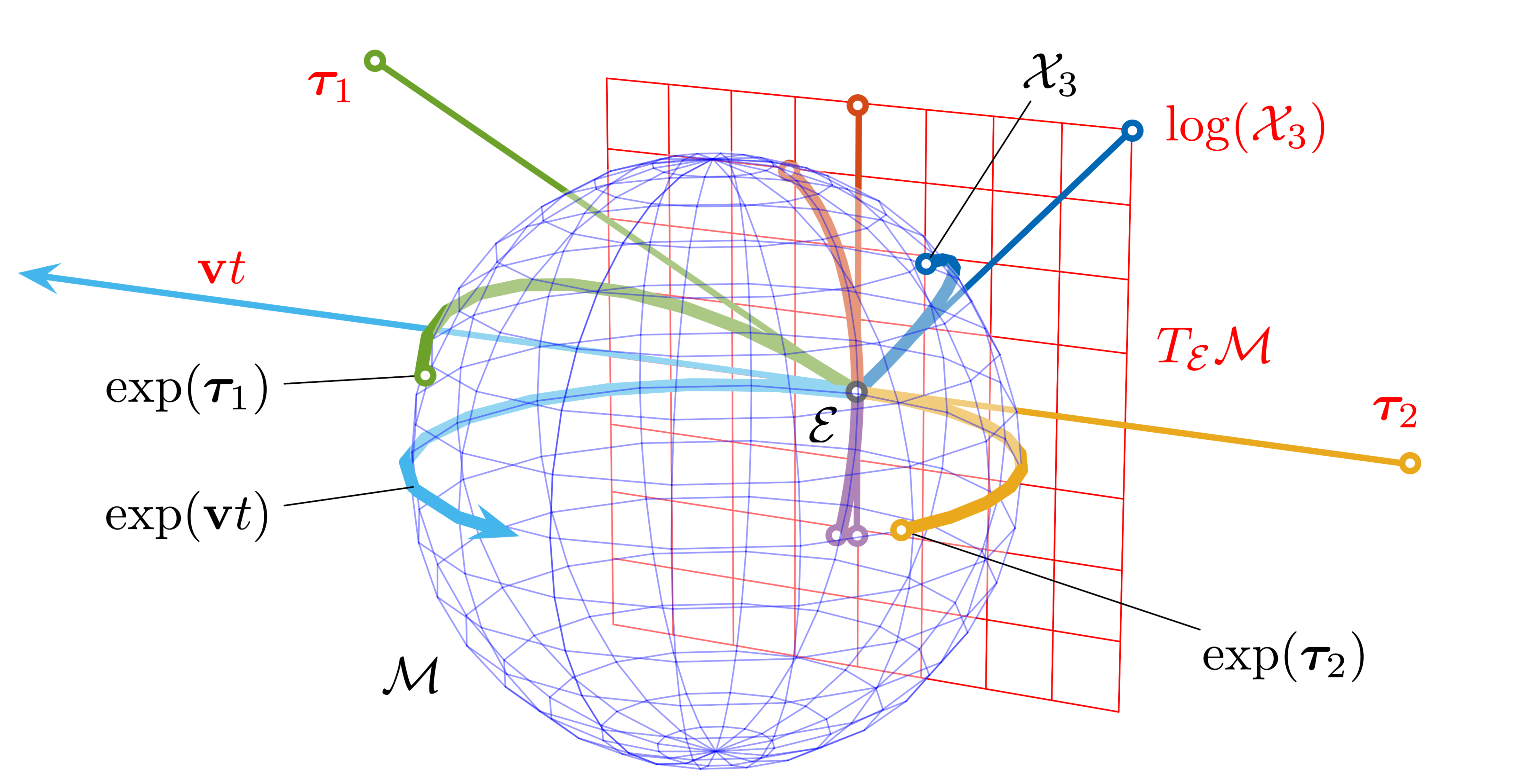
在单位元素附近的切空间$\mathrm{T}_{\mathcal{E}}\mathcal{M}$称为群$\mathcal{M}$的李代数$\mathcal{m}$,则: \(\begin{equation} \begin{aligned} \text{李代数} \hspace{1em} \mathcal{m} \triangleq \mathrm{T}_{\mathcal{E}}\mathcal{M} \end{aligned} \end{equation}\)
这里的$\mathcal{m}$是一个向量空间,它的元素可以被视为$\mathbb{R}$空间下的向量,$\mathcal{m}$的维度就是李群$\mathcal{M}$的自由度。而指数映射$exp$和对数映射$log$则是李群和李代数的相互转换方式,注意在这里的两个符号都是小写,表示的是李代数(切向量空间)上的元素转化,并不是所有维度下的向量都可以进行转换,我们在这里通常用$\land$帽子符号来说明李代数$\mathcal{m}$。为了方便我们直接在欧式空间$\mathbb{R}^3$上进行操作,所以我们还需要做欧式空间$\mathbb{R}^3$和李代数$\mathcal{m}$上的映射。依据群的特性(参考《SLAM十四讲》第三章
这里$\mathbf{e_{i}}$表示的是李代数$\mathcal{m}$下的基底,而$\mathbf{E_{i}}$是欧式空间下$\mathbb{R}^{m}$下的基底。所以我们可以定义欧式空间到李群的映射($\mathrm{Exp}$和$\mathrm{Log}$),即:
\[\begin{equation} \begin{aligned} \mathrm{Exp} &: \hspace{1em} \text{欧式空间}\mathbb{R}^{m} \rightarrow \mathcal{M} \hspace{1em} \mathcal{X} = Exp(\tau) \triangleq exp(\tau^{\land}) \\ \end{aligned} \end{equation}\] \[\begin{equation} \begin{aligned} \mathrm{Log} &: \hspace{1em} \mathcal{M} \rightarrow \text{欧式空间}\mathbb{R}^{m} \hspace{1em} \tau = Log(\mathcal{X}) \triangleq log(\mathcal{X})^{\vee} \\ \end{aligned} \end{equation}\]我们对公式(10)进行泰勒展开即可得到: \(\begin{equation} \begin{aligned} \mathcal{X} = exp(\tau^{\land}) = \mathcal{E} + \tau^{\land} + \frac{1}{2}\tau^{\land^{2}} + \frac{1}{3}\tau^{\land^{3}} + ... \\ \end{aligned} \end{equation}\) 在这里大家请记住公式(12),尤其当$\tau$是小量时,公式(12)可以简化为$exp(\tau^{\land}) \simeq \mathcal{E} + \tau^{\land}$是后面公式计算jacobian的重要工具之一。由于指数的性质,我们可以进一步得出李代数满足如下性质: $$ \begin{equation} \begin{aligned} \mathrm{exp((t+s)\tau^{\land})} = \mathrm{exp(t\tau^{\land})} \mathrm{exp(s\tau^{\land})}
\end{aligned} \end{equation}
\begin{equation} \begin{aligned} \mathrm{exp(t\tau^{\land})} = \mathrm{exp(\tau^{\land})^{t}}
\end{aligned} \end{equation}
\begin{equation} \begin{aligned} \mathrm{exp(-\tau^{\land})} = \mathrm{exp(\tau^{\land})^{-1}}
\end{aligned} \end{equation}
\begin{equation} \begin{aligned} \mathrm{exp(\mathcal{X}\tau^{\land}\mathcal{X}^{-1})} = \mathcal{X}\mathrm{exp(\tau^{\land})}\mathcal{X}^{-1}
\end{aligned} \end{equation} $$ 对此至此,我们对欧式空间、李代数和李群的基础定义介绍完毕。
机器人学中的李群/李代数运算
2.1 运算的方向
加法($ \oplus $)/减法($ \ominus $)是流形上用于表示运动递增/递减的常见运算之一。如图所示,每次的运算都是在当前点的切平面上。由于流形本身光滑的原因,由于当前点的切平面方向也在变化,造成的影响是每次递增或递减的方向也不同。所以对于群上来说左加还是右加,左减还是右减得到结果也都不同。
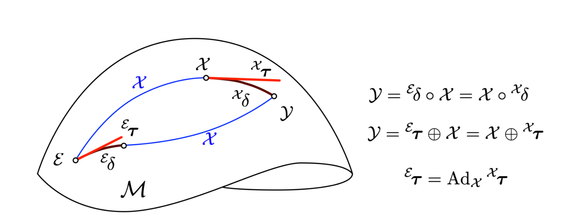
我们定义右加如下: $$ \begin{equation} \begin{aligned} \mathcal{Y} = \mathcal{X} \oplus {^{\mathcal{X}}\tau} \triangleq \mathcal{X} \circ \mathrm{Exp}({^{\mathcal{X}}\tau}) \in \mathcal{M}
\end{aligned} \end{equation}
\begin{equation} \begin{aligned} {^{\mathcal{X}}\tau} = \mathcal{Y} \ominus \mathcal{X} \triangleq Log(\mathcal{X}^{-1} \circ \mathcal{Y}) \in T_{\mathcal{X}}\mathcal{M}
\end{aligned} \end{equation} $$
需要注意的是这里${^{\mathcal{X}}\tau}$表示的应该是在$\mathcal{X}$点局部切平面上的无限小量。这里我们用左上标表示该小量所在的局部坐标系。从作者的粗浅理解来看,右运算在机器人学中相当于局部坐标系下的变化,对应的是四元数中的hamilton表示方式(这里粗浅的理解不一定正确,如果有错误,请及时拍砖并告诉我)。同理对应的左加/左减运算定义如下,这里小量是在全局坐标系下(我的理解对应的是四元数中的JPL表示方式): $$ \begin{equation} \begin{aligned} \mathcal{Y} = {^{\mathcal{E}}\tau} \oplus \mathcal{X} \triangleq \mathrm{Exp}({^{\mathcal{E}}\tau}) \circ \mathcal{X} \in \mathcal{M}
\end{aligned} \end{equation}
\begin{equation} \begin{aligned} {^{\mathcal{E}}\tau} = \mathcal{Y} \ominus \mathcal{X} \triangleq Log(\mathcal{Y} \circ \mathcal{X}^{-1} ) \in T_{\mathcal{E}}\mathcal{M}
\end{aligned} \end{equation} $$
2.2 伴随/伴随矩阵
由2.1,我们可知,李群本身并不满足交换律,所以机器人本身运动在局部坐标系下的递增幅度(右加)和全局坐标系下的递增幅度(左加)并不相同。由公式(17)和公式(19),我们可得:$ {^{\mathcal{E}}\tau} \oplus \mathcal{X} = \mathcal{X} \oplus {^{\mathcal{X}}\tau}$,并做如下递推: \(\begin{equation} \begin{aligned} \mathrm{Exp}({^{\mathcal{E}}\tau}) \mathcal{X} = \mathcal{X} \mathrm{Exp}({^{\mathcal{X}}\tau}) \\ \end{aligned} \end{equation}\)
\[\begin{equation} \begin{aligned} \mathrm{exp}({^{\mathcal{E}}\tau^{\land}}) = \mathcal{X} \mathrm{exp}({^{\mathcal{X}}\tau^{\land}}) \mathcal{X}^{-1} = \mathrm{exp}(\mathcal{X}{^{\mathcal{X}}\tau^{\land}}\mathcal{X}^{-1}) \\ \end{aligned} \end{equation}\] \[\begin{equation} \begin{aligned} {^{\mathcal{E}}\tau^{\land}} = \mathcal{X} {^{\mathcal{X}}\tau^{\land}} \mathcal{X}^{-1} \\ \end{aligned} \end{equation}\]如上所述,由公式(16)(21)(22),我们可以得到公式(23)。即局部坐标系下的增量与全局坐标系下的增量关系。因此我们可以定义状态$\mathcal{X}$的伴随如下: \(\begin{equation} \begin{aligned} \mathrm{Ad}_{\mathcal{X}}: \mathcal{m} \rightarrow \mathcal{m}\text{;} \hspace{1em} \tau^{\land} \rightarrow \mathrm{Ad}_{\mathcal{X}}(\tau^{\land}) \mathcal{X} {^{\mathcal{X}}\tau^{\land}} \mathcal{X}^{-1} \\ \end{aligned} \end{equation}\) 需要注意的是这里的伴随符号$\mathrm{Ad}_{\mathcal{X}}$并没有加粗,表示的是在李代数上的运算,依据定义我们可知在李代数$\mathcal{m}$上的伴随具有如下性质: \(\begin{equation} \begin{aligned} \text{齐次性:} \mathrm{Ad}_{\mathcal{X}}(a\tau^{\land} + b\sigma^{\land})= a\mathrm{Ad}_{\mathcal{X}}(\tau^{\land}) + b \mathrm{Ad}_{\mathcal{X}}(\sigma^{\land}) \\ \end{aligned} \end{equation}\)
\[\begin{equation} \begin{aligned} \text{同态:} \mathrm{Ad}_{\mathcal{X}}(\mathrm{Ad}_{\mathcal{Y}}(\tau^{\land}))= \mathrm{Ad}_{\mathcal{XY}}(\tau^{\land})\\ \end{aligned} \end{equation}\]对应的,在欧式空间$\mathbb{R}$下的伴随矩阵则定义如下: \(\begin{equation} \begin{aligned} \mathbf{Ad}_{\mathcal{X}}: \mathbb{R}^m \rightarrow \mathbb{R}^m\text{;} \hspace{1em} {^{\mathcal{X}}\tau^{\land}} \rightarrow {^{\mathcal{E}}\tau^{\land}} = \mathbf{Ad}_{\mathcal{X}}{^{\mathcal{X}}\tau^{\land}} \\ \end{aligned} \end{equation}\)
注意到这里的$\mathbf{Ad}_{\mathcal{X}}$是加粗的,表示在欧式空间$\mathbb{R}$上的操作,依据定义,我们还能得到如下性质: \(\begin{equation} \begin{aligned} \mathcal{X} \oplus \tau = (\mathbf{Ad}_{\mathcal{X}}\tau) \oplus \mathcal{X} \\ \end{aligned} \end{equation}\)
\[\begin{equation} \begin{aligned} \mathbf{Ad}_{\mathcal{X}^{-1}} = \mathbf{Ad}_{\mathcal{X}}^{-1} \\ \end{aligned} \end{equation}\]\(\begin{equation} \begin{aligned} \mathbf{Ad}_{\mathcal{X}\mathcal{Y}} = \mathbf{Ad}_{\mathcal{X}} \mathbf{Ad}_{\mathcal{Y}} \\ \end{aligned} \end{equation}\) 到此,我们有关李群上的运算基本介绍完成,下面开始介绍开发者最头疼的部分李群/李代数上的导数。
2.3 李群上的导数
回顾下导数的定义,当我们对一个函数求导的时候,求导方式定义如下: \(\begin{equation} \mathbf{J} = \frac{\partial f(\mathbf{x})}{\partial \mathbf{x}} \triangleq \lim_{\mathbf{h} \rightarrow 0} \frac{f(\mathbf{x}+\mathbf{h}) - f(\mathbf{x})}{\mathbf{x}} \in \mathbb{R} \end{equation}\) 由于我们前面提过群本身是流形且光滑,所以基于上式,我们基本上可以推导出机器人学中常用的jacobian,定义如下: \(\begin{equation} \frac{^{\mathcal{X}}Df(\mathcal{X})}{D\mathcal{X}} = \lim_{\tau \rightarrow 0} \frac{f(\mathcal{X} \oplus \tau) \ominus f(\mathcal{X})}{\tau} \in \mathbb{R} \end{equation}\)
如前文所述,我们将在下面着重对$SO(3)$旋转群和$SE(3)$运动群进行推导。
2.3.1 SO(3)群上导数
$SO(3)+\mathbf{t}$是激光SLAM中最常用的位姿表现形式,其中点的变化是一系列推导工作的基础。我们在这里就针对这个问题来进行jacobian推导。这里位姿$\mathbf{T} = [\mathbf{R}, \mathbf{t}]$,则点的变化为$f(\mathbf{T}) = \mathbf{R} \mathbf{P} + \mathbf{t}$,对此我们可以通过右扰动求导如下: \(\begin{equation} \begin{aligned} \frac{^{\mathbf{R}}D(\mathbf{R}\mathbf{P}+\mathbf{t})}{D\mathbf{R}} &= \lim_{\theta \rightarrow 0} \frac{[(\mathbf{R} \oplus \mathbf{\theta})\mathbf{P} + \mathbf{t}] \ominus f(\mathbf{T})}{\mathbf{\theta}} \\ &= \lim_{\theta \rightarrow 0} \frac{[(\mathbf{R} \mathbf{Exp}(\theta))\mathbf{P} + \bcancel{\mathbf{t}}] - [\mathbf{R}\mathbf{P} + \bcancel{\mathbf{t}}]}{\theta} \\ &\simeq \frac{[\mathbf{R}(\bcancel{\mathbf{I}} + [\mathbf{\theta}]_{\times})\mathbf{P}] - \bcancel{\mathbf{R}\mathbf{P}}}{\theta} = \frac{\mathbf{R}[\mathbf{\theta}]_{\times}\mathbf{P}}{\mathbf{\theta}} \\ &= \lim_{\theta \rightarrow 0} \frac{-\mathbf{R}[\mathbf{P}]_{\times}\mathbf{\theta}}{\mathbf{\theta}} \\ &= -\mathbf{R}[\mathbf{P}]_{\times} \in \mathbb{R}^{3 \times 3} \end{aligned} \end{equation}\) 需要注意,在这里推导的时候$\mathbf{\theta}$应该是接近于0的无限小量,这样才能满足之前提到的公式(12)要求,对整体做近似。对此,我们对$SO(3)$的群进行右扰动求导完成。当然对SO(3)也可以进行左扰动求导(因为当日写公式时间太久,所以暂时不做推导,后续补上)。
2.3.2 SE(3)群上导数
类似于上面的$SO(3)$群,我们也可以通过右扰动对$SE(3)$进行Jacobian求解。考虑到《SLAM十四讲》
对此,关于$SO(3)$和$SE(3)$的Jacobian解析式求导已完成。如前言里说的一样,基于李群的解析式求导在目前的很多SLAM系统中都能看到:如$SO(3)$求导在港大的Fast-LIO
数值差分Jacobian及其代码实现
我在博一的时候,实验室邹丹平老师就经常和我说:“别在纸上推啦,推又推不对,推对了又写错,有啥用,还不如直接差分求导”。

我不知道怎么和他开口说,不是我不想用,而是我不会。有次好不容易鼓起勇气问他,他:“哇靠,这都不会,看我PPT第28页,写的不能再清楚了”。
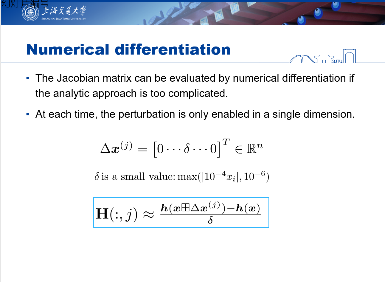
在那个时候我明白了,高手眼里的世界和我们菜狗眼里的世界是不一样的。现在我博五,回过头来看,明白是自己当初对公式(31)理解不够深入的,下面我们来对公式代码化:用Sophus库来表示当前状态。矩阵操作依赖Eigen库来实现,主要对上面的$SO(3)$群的例子进行数值Jacobian求导。 回顾PPT里,这里最主要需要实现的就是优化函数(cost function):即$\mathbf{R}\mathbf{P}+\mathbf{t}$。剩下的就是定义小量,计算优化函数变化,得到的就是对应的数值差分jacobian,C++伪代码定义如下(这里我们主要考虑的就是旋转,平移部分做相同操作即可):
// 定义小量:
double delta = 1e-7;
// Map the delta into the rotation.
for(i = 0; i < 3; ++i) {
  Eigen::Vector3d delta_vector = Eigen::Vector3d::Zero();
  delta_vector(i) = delta;
  // current_state是我们定义机器人状态量,包含机器人当前姿态和位置。
  Sophus::SO3d delta_rotation = current_state.rotation * Sophus::SO3d::exp(delta_vector);
  Eigen::Vector3d delta_map_point = delta_rotation * point + current_state.position;
  Eigen::Vector3d delta_error = ( delta_map_point  - current_map_point);
  Eigen::Vector3d num_diff_vector = delta_error / delta;
  LOG(INFO) << num_diff_vector.transpose();
}
通过代码不难看出,差分求jacobian实际上就是对每一个部分进行小扰动后看整体优化函数的变化幅度(也就是微分的定义)。从开发的角度来看,这种方式的确在SLAM工程初期能快速地求解出jacobian。虽然该方法实际运行效率相对较低,但是我们可以在初期使用,后期在整体系统构建完成后,再用解析式求导来加速,这时差分方法也可以来验证这里的变化。但是差分的作用不仅仅如此,更精彩的妙用是在左星星老师CodeVIO中的妙用,通过差分的方式来求解出CVAE的Jacobian。这篇论文也被ICRA2021提名为Robot Vsion方向的最佳论文,十分推荐大家去读读。说到深度学习,那李群和李代数在深度学习中又是怎么样呢?这里我就推荐CMU Chen wang老师的PyPose
总结。
本篇Blog我们回顾了李群的定义和数值差分求导的实现方式,希望能更好地帮助到SLAM研究者们能更快更好的构建自己的SLAM系统,最起码不会被Jacobian求解给难住。如果觉得我哪里写错或者不够清楚,欢迎email或评论区说出你的想法。